Excel’s What-If Analysis tool is broken down into three main components. The part discussed here is the powerful Goal Seek feature that lets you work backwards from a function and determine the inputs necessary to get the desired output from a formula in a cell. Read on to learn how to use Excel’s What-If Analysis Goal Seek tool.
Excel’s Goal Seek Tool Example
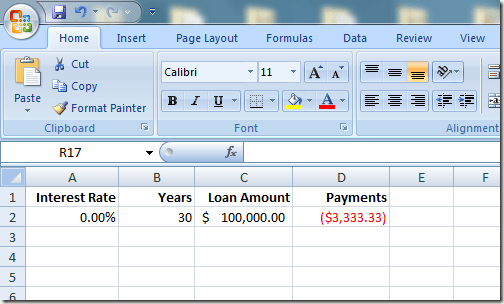
Suppose that you want to take out a mortgage loan to buy a house and you are concerned about how the interest rate on the loan will affect the yearly payments. The amount of the mortgage is $100,000 and you will pay back the loan over the course of 30 years. Using Excel’s PMT function, you can easily figure out what the yearly payments would be if the interest rate were 0%. The spreadsheet would likely look something like this:
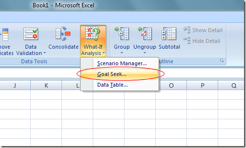
The cell at A2 represents the yearly interest rate, the cell at B2 is the length of the loan in years, and the cell at C2 is the amount of the mortgage loan. The formula in D2 is: and represents the yearly payments of a 30-year, $100,000 mortgage at 0% interest. Notice that the figure in D2 is negative since Excel assumes that the payments are a negative cash flow from your financial position. Unfortunately, no mortgage lender is going to lend you $100,000 at 0% interest. Suppose you do some figuring and find out that you can afford to pay back $6,000 per year in mortgage payments. You are now wondering what is the highest interest rate you can take on for the loan to make sure you don’t end up paying more than $6,000 per year. Many people in this situation would simply start typing numbers in cell A2 until the figure in D2 reached approximately $6,000. However, you can make Excel do the work for you by using the What-If Analysis Goal Seek tool. Essentially, you will make Excel work backwards from the result in D4 until it arrives at an interest rate that satisfies your maximum payout of $6,000. Begin by clicking on the Data tab on the Ribbon and locating the What-If Analysis button in the Data Tools section. Click on the What-If Analysis button and choose Goal Seek from the menu.
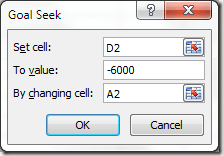
Excel opens up a small window and asks you to input only three variables. The Set Cell variable must be a cell that contains a formula. In our example here, it is D2. The To Value variable is the amount you want the cell at D2 to be at the end of the analysis. For us, it is -6,000. Remember that Excel sees payments as a negative cash flow. The By Changing Cell variable is the interest rate you want Excel to find for you so that the $100,000 mortgage will cost you only $6,000 per year. So, use cell A2.
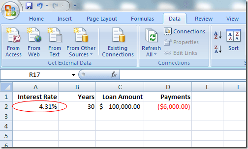
Click the OK button and you may notice that Excel flashes a bunch of numbers in the respective cells until the iterations finally converge on a final number. In our case, the cell at A2 should now read about 4.31%.
This analysis tells us that in order not to spend more than $6,000 per year on a 30-year, $100,000 mortgage, you need to secure the loan at no more than 4.31%. If you want to continue doing what-if analyses, you can try different combinations of numbers and variables to explore the options you have when trying to secure a good interest rate on a mortgage. Excel’s What-If Analysis Goal Seek tool is a powerful complement to the various functions and formulas found in the typical spreadsheet. By working backwards from the results of a formula in a cell, you can explore the different variables in your calculations more clearly.


